1. 簡介
在本程式碼研究室中,您將訓練模型,根據一組汽車的數值型資料進行預測。
本練習將示範訓練多種不同模型時的常見步驟,但會使用小型資料集和簡單 (淺層) 模型。主要目標是協助您熟悉使用 TensorFlow.js 訓練模型的基本術語、概念和語法,並為進一步探索和學習奠定基礎。
由於我們訓練模型是為了預測連續數字,因此這項工作有時也稱為「迴歸」工作。我們會向模型展示許多輸入內容和正確輸出內容的範例,藉此訓練模型。這就是所謂的監督式學習。
建構目標
您將建立網頁,使用 TensorFlow.js 在瀏覽器中訓練模型。模型會根據車輛的「馬力」預測「每加侖英里數」(MPG)。
做法如下:
- 載入資料並準備用於訓練。
- 定義模型架構。
- 訓練模型並監控訓練期間的效能。
- 進行一些預測,評估訓練好的模型。
課程內容
- 機器學習資料準備的最佳做法,包括隨機排序和正規化。
- 使用 tf.layers API 建立模型的 TensorFlow.js 語法。
- 如何使用 tfjs-vis 程式庫監控瀏覽器內訓練。
軟硬體需求
- 使用新版 Chrome 或其他新式瀏覽器。
- 文字編輯器,可在本機電腦上執行,也可以透過 Codepen 或 Glitch 等服務在網路上執行。
- 熟悉 HTML、CSS、JavaScript 和 Chrome 開發人員工具 (或您偏好的瀏覽器開發人員工具)。
- 對類神經網路有高階概念性瞭解。如需簡介或複習,建議觀看 3blue1brown 的這部影片,或是 Ashi Krishnan 的這部 JavaScript 深度學習影片。
2. 做好準備
建立 HTML 網頁並加入 JavaScript
 將下列程式碼複製到名為 的 html 檔案中
index.html
<!DOCTYPE html>
<html>
<head>
  <title>TensorFlow.js Tutorial</title>

  <!-- Import TensorFlow.js -->
  <script src="https://cdn.jsdelivr.net/npm/@tensorflow/tfjs@2.0.0/dist/tf.min.js"></script>
  <!-- Import tfjs-vis -->
  <script src="https://cdn.jsdelivr.net/npm/@tensorflow/tfjs-vis@1.0.2/dist/tfjs-vis.umd.min.js"></script>
</head>
<body>
  <!-- Import the main script file -->
  <script src="script.js"></script>
</body>
</html>
建立程式碼的 JavaScript 檔案
- 在與上述 HTML 檔案相同的資料夾中,建立名為 script.js 的檔案,並在其中加入下列程式碼。
console.log('Hello TensorFlow');
立即測試
現在您已建立 HTML 和 JavaScript 檔案,請測試這些檔案。在瀏覽器中開啟 index.html 檔案,並開啟開發人員工具控制台。
如果一切正常,開發人員工具控制台應該會建立並提供兩個全域變數:
tf是指 TensorFlow.js 程式庫tfvis是指 tfjs-vis 程式庫
開啟瀏覽器的開發人員工具,您應該會在控制台輸出內容中看到 Hello TensorFlow 訊息。如果是,即可繼續下一個步驟。
3. 載入、格式化及以圖表呈現輸入資料
首先,請載入、格式化並視覺化要用來訓練模型的資料。
我們會從為您代管的 JSON 檔案載入「cars」資料集。其中包含每輛車的許多不同功能。在本教學課程中,我們只想擷取馬力和每加侖英里數的資料。
將下列程式碼加到
script.js 檔案
/**
 * Get the car data reduced to just the variables we are interested
 * and cleaned of missing data.
 */
async function getData() {
  const carsDataResponse = await fetch('https://storage.googleapis.com/tfjs-tutorials/carsData.json');
  const carsData = await carsDataResponse.json();
  const cleaned = carsData.map(car => ({
    mpg: car.Miles_per_Gallon,
    horsepower: car.Horsepower,
  }))
  .filter(car => (car.mpg != null && car.horsepower != null));

  return cleaned;
}
系統也會移除未定義每加侖英里數或馬力的項目。我們也將這些資料繪製成散佈圖,看看會呈現什麼樣貌。
將下列程式碼新增至 底部:
script.js file.
async function run() {
  // Load and plot the original input data that we are going to train on.
  const data = await getData();
  const values = data.map(d => ({
    x: d.horsepower,
    y: d.mpg,
  }));

  tfvis.render.scatterplot(
    {name: 'Horsepower v MPG'},
    {values},
    {
      xLabel: 'Horsepower',
      yLabel: 'MPG',
      height: 300
    }
  );

  // More code will be added below
}

document.addEventListener('DOMContentLoaded', run);
重新整理頁面時,頁面左側應會顯示資料的散佈圖。看起來應該會像這樣
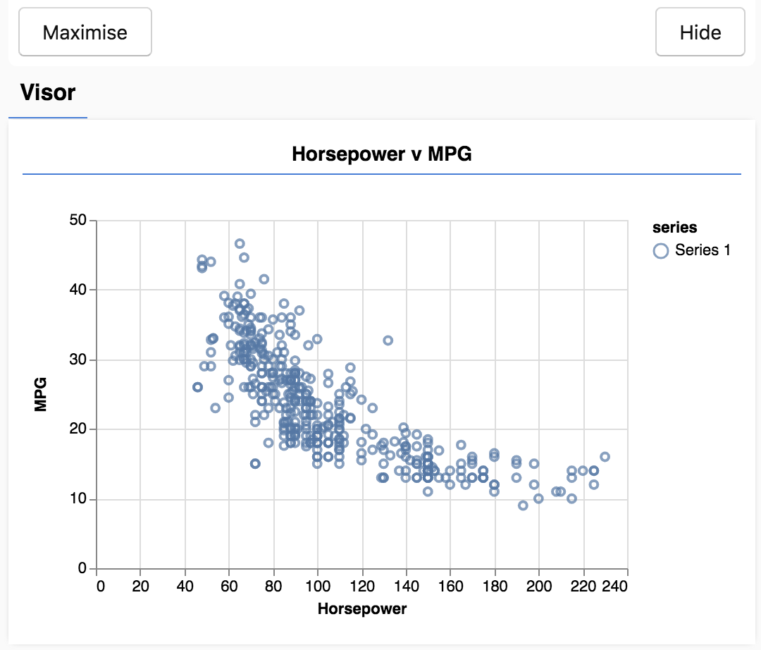
這個面板稱為遮陽板,由 tfjs-vis 提供。方便您顯示視覺化內容。
一般來說,處理資料時最好找出查看資料的方式,並視需要清理資料。在這種情況下,我們必須從 carsData 中移除缺少必要欄位的項目。將資料視覺化,有助於判斷資料是否具有模型可學習的結構。
從上圖可以看出,馬力和每加侖汽油可行駛里程數之間呈現負相關,也就是說,馬力越大,每加侖汽油可行駛里程數就越少。
構思工作
輸入資料現在會如下所示。
...
{
  "mpg":15,
  "horsepower":165,
},
{
  "mpg":18,
  "horsepower":150,
},
{
  "mpg":16,
  "horsepower":150,
},
...
我們的目標是訓練模型,讓模型接收一個數字 (即「馬力」),並學會預測一個數字 (即「每加侖英里數」)。請記住一對一對應關係,因為這對下一節很重要。
我們將這些範例 (馬力和每加侖汽油可行駛里程數) 輸入類神經網路,讓網路從這些範例中學習公式 (或函式),根據馬力預測每加侖汽油可行駛里程數。這種從有正確答案的範例中學習的過程,稱為監督式學習。
4. 定義模型架構
在本節中,我們將編寫程式碼來描述模型架構。模型架構只是「模型執行時會執行的函式」或「模型會使用哪種演算法計算答案」的另一種說法。
機器學習模型是演算法,可接收輸入內容並產生輸出內容。使用類神經網路時,演算法是一組神經元層,其中「權重」(數字) 會控管輸出內容。訓練程序會找出這些權重的理想值。
在 中新增下列函式
script.js 檔案,用於定義模型架構。
function createModel() {
  // Create a sequential model
  const model = tf.sequential();

  // Add a single input layer
  model.add(tf.layers.dense({inputShape: [1], units: 1, useBias: true}));

  // Add an output layer
  model.add(tf.layers.dense({units: 1, useBias: true}));

  return model;
}
這是我們可以在 tensorflow.js 中定義的最簡單模型之一,讓我們稍微分析每一行。
例項化模型
const model = tf.sequential();
這會建立 tf.Model 物件的例項。這個模型是 sequential,因為輸入內容會直接流向輸出內容。其他類型的模型可以有分支,甚至可以有多個輸入和輸出,但在許多情況下,模型會是循序的。序列模型也更容易使用 API。
新增圖層
model.add(tf.layers.dense({inputShape: [1], units: 1, useBias: true}));
這會在網路中新增輸入層,並自動連結至具有一個隱藏單元的 dense 層。dense 層是一種層,會將輸入內容乘以矩陣 (稱為「權重」),然後在結果中加入數字 (稱為「偏差」)。由於這是網路的第一層,因此我們需要定義 inputShape。由於我們將 1 數值 (特定車輛的馬力) 做為輸入內容,因此 inputShape 為 [1]。
units 會設定圖層中的權重矩陣大小。在此將其設為 1,表示資料的每個輸入特徵都會有 1 個權重。
model.add(tf.layers.dense({units: 1}));
上方程式碼會建立輸出層。我們將 units 設為 1,因為我們想要輸出 1 個數字。
建立執行個體
在 中加入下列程式碼:
run 我們稍早定義的函式。
// Create the model
const model = createModel();
tfvis.show.modelSummary({name: 'Model Summary'}, model);
這會建立模型執行個體,並在網頁上顯示圖層摘要。
5. 準備訓練資料
如要充分發揮 TensorFlow.js 的效能,讓訓練機器學習模型成為可行的做法,我們需要將資料轉換為張量。我們也會對資料執行多項最佳做法的轉換作業,也就是隨機排序和正規化。
將下列程式碼加到
script.js 檔案
/**
 * Convert the input data to tensors that we can use for machine
 * learning. We will also do the important best practices of _shuffling_
 * the data and _normalizing_ the data
 * MPG on the y-axis.
 */
function convertToTensor(data) {
  // Wrapping these calculations in a tidy will dispose any
  // intermediate tensors.

  return tf.tidy(() => {
    // Step 1. Shuffle the data
    tf.util.shuffle(data);

    // Step 2. Convert data to Tensor
    const inputs = data.map(d => d.horsepower)
    const labels = data.map(d => d.mpg);

    const inputTensor = tf.tensor2d(inputs, [inputs.length, 1]);
    const labelTensor = tf.tensor2d(labels, [labels.length, 1]);

    //Step 3. Normalize the data to the range 0 - 1 using min-max scaling
    const inputMax = inputTensor.max();
    const inputMin = inputTensor.min();
    const labelMax = labelTensor.max();
    const labelMin = labelTensor.min();

    const normalizedInputs = inputTensor.sub(inputMin).div(inputMax.sub(inputMin));
    const normalizedLabels = labelTensor.sub(labelMin).div(labelMax.sub(labelMin));

    return {
      inputs: normalizedInputs,
      labels: normalizedLabels,
      // Return the min/max bounds so we can use them later.
      inputMax,
      inputMin,
      labelMax,
      labelMin,
    }
  });
}
讓我們來分析一下這裡發生了什麼事。
隨機取用資料
// Step 1. Shuffle the data
tf.util.shuffle(data);
在這裡,我們會隨機排列要提供給訓練演算法的範例順序。洗牌很重要,因為在訓練期間,資料集通常會分成較小的子集 (稱為批次),模型會根據這些子集進行訓練。這樣一來,每個批次都會包含資料分佈中的各種資料。這麼做有助於模型:
- 不會學習純粹取決於資料輸入順序的內容
- 對子群組中的結構不敏感 (例如,如果模型在訓練的前半段只看到高馬力的車輛,可能會學到不適用於資料集其餘部分的關係)。
轉換為張量
// Step 2. Convert data to Tensor
const inputs = data.map(d => d.horsepower)
const labels = data.map(d => d.mpg);

const inputTensor = tf.tensor2d(inputs, [inputs.length, 1]);
const labelTensor = tf.tensor2d(labels, [labels.length, 1]);
我們在這裡建立兩個陣列,一個用於輸入範例 (馬力項目),另一個用於真實輸出值 (在機器學習中稱為標籤)。
然後將每個陣列資料轉換為 2D 張量。張量的形狀為 [num_examples, num_features_per_example]。這裡有 inputs.length 個範例,每個範例都有 1 個輸入特徵 (馬力)。
將資料標準化
//Step 3. Normalize the data to the range 0 - 1 using min-max scaling
const inputMax = inputTensor.max();
const inputMin = inputTensor.min();
const labelMax = labelTensor.max();
const labelMin = labelTensor.min();

const normalizedInputs = inputTensor.sub(inputMin).div(inputMax.sub(inputMin));
const normalizedLabels = labelTensor.sub(labelMin).div(labelMax.sub(labelMin));
接下來,我們將介紹另一個機器學習訓練最佳做法。我們正規化資料。這裡我們使用 min-max 縮放,將資料正規化為 0-1 數值範圍。正規化非常重要,因為您使用 tensorflow.js 建構的許多機器學習模型內部,都是設計用來處理不太大的數字。正規化資料的常見範圍包括 0 to 1 或 -1 to 1。如果養成將資料正規化至合理範圍的習慣,訓練模型時會更加得心應手。
傳回資料和正規化界限
return {
  inputs: normalizedInputs,
  labels: normalizedLabels,
  // Return the min/max bounds so we can use them later.
  inputMax,
  inputMin,
  labelMax,
  labelMin,
}
我們希望保留訓練期間用於正規化的值,這樣就能將輸出結果反正規化,還原為原始比例,並以相同方式正規化未來的輸入資料。
6. 訓練模型
建立模型執行個體並以張量表示資料後,我們已準備好開始訓練程序。
將下列函式複製到
script.js file.
async function trainModel(model, inputs, labels) {
  // Prepare the model for training.
  model.compile({
    optimizer: tf.train.adam(),
    loss: tf.losses.meanSquaredError,
    metrics: ['mse'],
  });

  const batchSize = 32;
  const epochs = 50;

  return await model.fit(inputs, labels, {
    batchSize,
    epochs,
    shuffle: true,
    callbacks: tfvis.show.fitCallbacks(
      { name: 'Training Performance' },
      ['loss', 'mse'],
      { height: 200, callbacks: ['onEpochEnd'] }
    )
  });
}
讓我們來詳細說明。
準備訓練
// Prepare the model for training.
model.compile({
  optimizer: tf.train.adam(),
  loss: tf.losses.meanSquaredError,
  metrics: ['mse'],
});
我們必須先「編譯」模型,才能訓練模型。為此,我們必須指定許多非常重要的事項:
optimizer:這是管理模型更新的演算法,會隨著模型查看範例而更新。TensorFlow.js 提供許多最佳化工具。我們在此選取了 adam 最佳化工具,因為這個工具在實務上相當有效,而且不需要任何設定。loss:這個函式會告訴模型,在學習顯示的每個批次 (資料子集) 時,模型的表現如何。在這裡,我們使用meanSquaredError比較模型預測值與真實值。
const batchSize = 32;
const epochs = 50;
接著,我們選取 batchSize 和 epoch 數量:
batchSize是指模型在每次訓練疊代中看到的資料子集大小。常見的批次大小通常介於 32 到 512 之間。所有問題都沒有理想的批量大小,而且本教學課程的範圍不包括說明各種批量大小的數學動機。epochs是指模型查看您提供的整個資料集的次數。這裡我們會對資料集進行 50 次疊代。
開始訓練迴圈
return await model.fit(inputs, labels, {
  batchSize,
  epochs,
  callbacks: tfvis.show.fitCallbacks(
    { name: 'Training Performance' },
    ['loss', 'mse'],
    { height: 200, callbacks: ['onEpochEnd'] }
  )
});
model.fit 是我們呼叫的函式,用來啟動訓練迴圈。這是非同步函式,因此我們會傳回函式提供的 Promise,讓呼叫端判斷訓練何時完成。
如要監控訓練進度,我們會將一些回呼傳遞至 model.fit。我們會使用 tfvis.show.fitCallbacks 產生函式,繪製先前指定的「loss」和「mse」指標圖表。
綜合應用範例
現在,我們必須從 run 函式呼叫已定義的函式。
將下列程式碼新增至 底部:
run 函式。
// Convert the data to a form we can use for training.
const tensorData = convertToTensor(data);
const {inputs, labels} = tensorData;

// Train the model
await trainModel(model, inputs, labels);
console.log('Done Training');
重新整理頁面後,您應該會在幾秒內看到下列圖表更新。
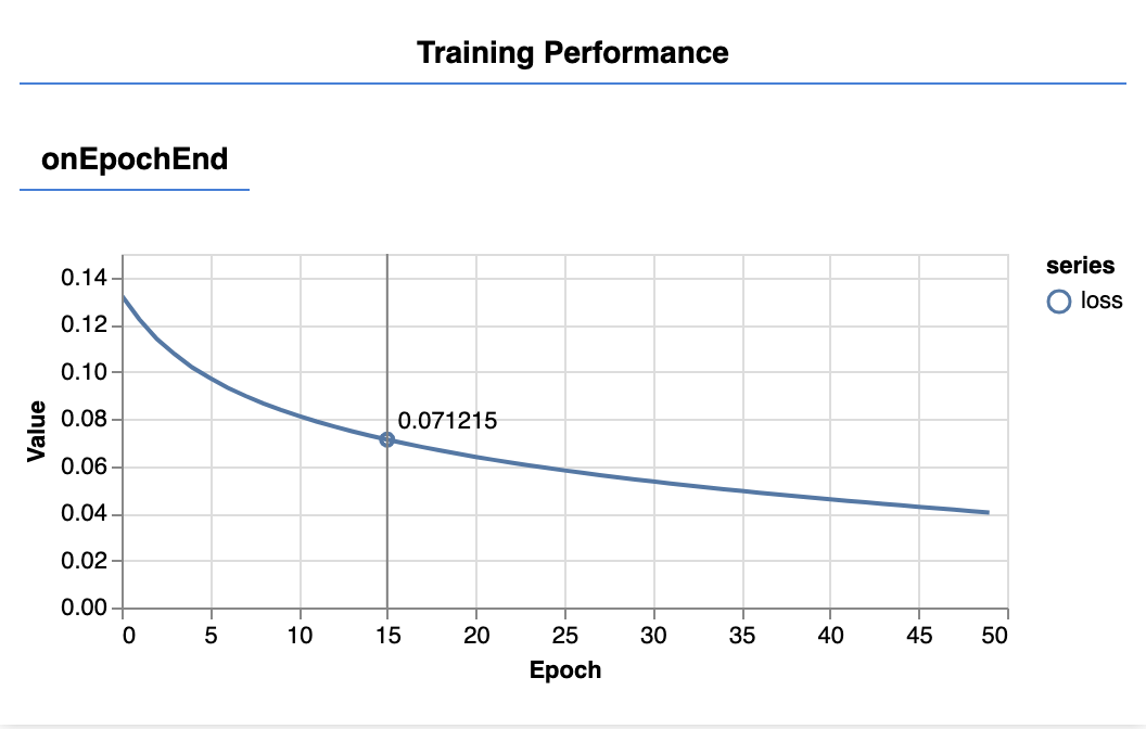
這些是先前建立的回呼所建立的。在每個訓練週期結束時,這些指標會顯示整個資料集的平均損失和 MSE。
訓練模型時,我們希望損失會降低。在本例中,由於我們的指標是錯誤的測量結果,因此我們也希望看到指標下降。
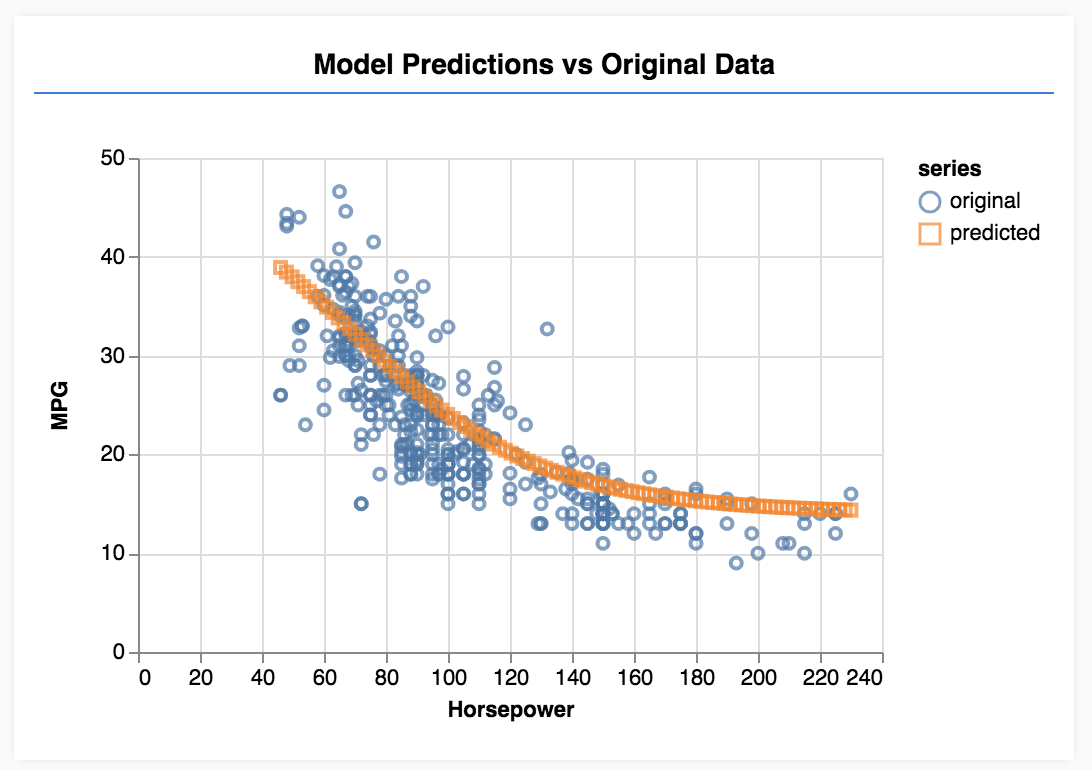
7. 進行預測
模型訓練完成後,我們想進行一些預測。讓我們評估模型,看看模型對馬力從低到高的統一範圍預測結果。
將下列函式新增至 script.js 檔案
function testModel(model, inputData, normalizationData) {
  const {inputMax, inputMin, labelMin, labelMax} = normalizationData;

  // Generate predictions for a uniform range of numbers between 0 and 1;
  // We un-normalize the data by doing the inverse of the min-max scaling
  // that we did earlier.
  const [xs, preds] = tf.tidy(() => {

    const xsNorm = tf.linspace(0, 1, 100);
    const predictions = model.predict(xsNorm.reshape([100, 1]));

    const unNormXs = xsNorm
      .mul(inputMax.sub(inputMin))
      .add(inputMin);

    const unNormPreds = predictions
      .mul(labelMax.sub(labelMin))
      .add(labelMin);

    // Un-normalize the data
    return [unNormXs.dataSync(), unNormPreds.dataSync()];
  });


  const predictedPoints = Array.from(xs).map((val, i) => {
    return {x: val, y: preds[i]}
  });

  const originalPoints = inputData.map(d => ({
    x: d.horsepower, y: d.mpg,
  }));


  tfvis.render.scatterplot(
    {name: 'Model Predictions vs Original Data'},
    {values: [originalPoints, predictedPoints], series: ['original', 'predicted']},
    {
      xLabel: 'Horsepower',
      yLabel: 'MPG',
      height: 300
    }
  );
}
請注意上述函式中的幾項事項。
const xsNorm = tf.linspace(0, 1, 100);
const predictions = model.predict(xsNorm.reshape([100, 1]));
我們會產生 100 個新「範例」,提供給模型。我們就是透過 Model.predict 將這些範例輸入模型。請注意,這些資料的形狀必須與訓練時的形狀 ([num_examples, num_features_per_example]) 相似。
// Un-normalize the data
const unNormXs = xsNorm
  .mul(inputMax.sub(inputMin))
  .add(inputMin);

const unNormPreds = predictions
  .mul(labelMax.sub(labelMin))
  .add(labelMin);
如要將資料還原至原始範圍 (而非 0 到 1),請使用我們在正規化時計算的值,但只要反向操作即可。
return [unNormXs.dataSync(), unNormPreds.dataSync()];
.dataSync() 是一種方法,可用於取得儲存在張量中的值 typedarray。這樣我們就能在一般 JavaScript 中處理這些值。這是 .data() 方法的同步版本,一般來說較為建議。
最後,我們使用 tfjs-vis 繪製原始資料和模型預測結果。
將下列程式碼加到
run 函式。
// Make some predictions using the model and compare them to the
// original data
testModel(model, data, tensorData);
重新整理頁面,模型訓練完成後,您應該會看到類似下列內容的畫面。
恭喜!您剛訓練了一個簡單的機器學習模型。目前會執行所謂的線性迴歸,嘗試在輸入資料中找出趨勢並繪製成線。
8. 主要重點
訓練機器學習模型的步驟包括:
擬定工作:
- 這是迴歸問題還是分類問題?
- 這項工作可以透過監督式學習或非監督式學習完成嗎?
- 輸入資料的形狀為何?輸出資料應為何種格式?
準備資料:
- 盡可能清理資料並手動檢查模式
- 先隨機排序資料,再用於訓練
- 將資料正規化至類神經網路的合理範圍。通常 0 到 1 或 -1 到 1 是數值型資料的合適範圍。
- 將資料轉換為張量
建構及執行模型:
- 使用
tf.sequential或tf.model定義模型,然後使用tf.layers.*在模型中新增圖層 - 選擇最佳化器 ( 通常 adam 是不錯的選擇),以及批量和訓練週期數等參數。
- 為問題選擇適當的損失函式,以及有助於評估進度的準確度指標。
meanSquaredError是迴歸問題的常見損失函式。 - 監控訓練,確認損失是否下降
評估模型
- 為模型選擇評估指標,以便在訓練期間監控。訓練完成後,請嘗試進行一些測試預測,瞭解預測品質。
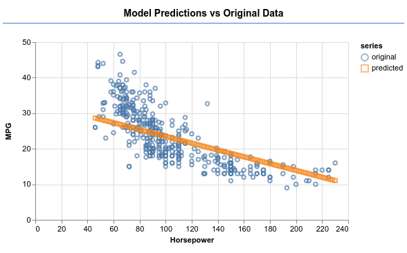
9. 額外學分:值得一試的操作
- 實驗變更訓練週期數。圖表趨於平緩前,您需要多少個訓練週期。
- 嘗試增加隱藏層中的單元數。
- 實驗看看在我們新增的第一個隱藏層和最終輸出層之間,加入更多隱藏層。這些額外圖層的程式碼應如下所示。
model.add(tf.layers.dense({units: 50, activation: 'sigmoid'}));
這些隱藏層最重要的創新之處,在於導入非線性活化函數,也就是 sigmoid 活化函數。如要進一步瞭解啟用函式,請參閱這篇文章。
看看模型是否能產生如下圖所示的輸出內容。